The Trouble with the Purple Election Map

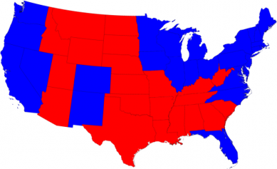
Every 4 years, we’re given a map like this:

Usually, a dissatisfied data visualizer is less than thrilled with entire states being designated as either red or blue. The analyst, wanting a clearer picture of the political landscape, breaks the original map down to a county-level:

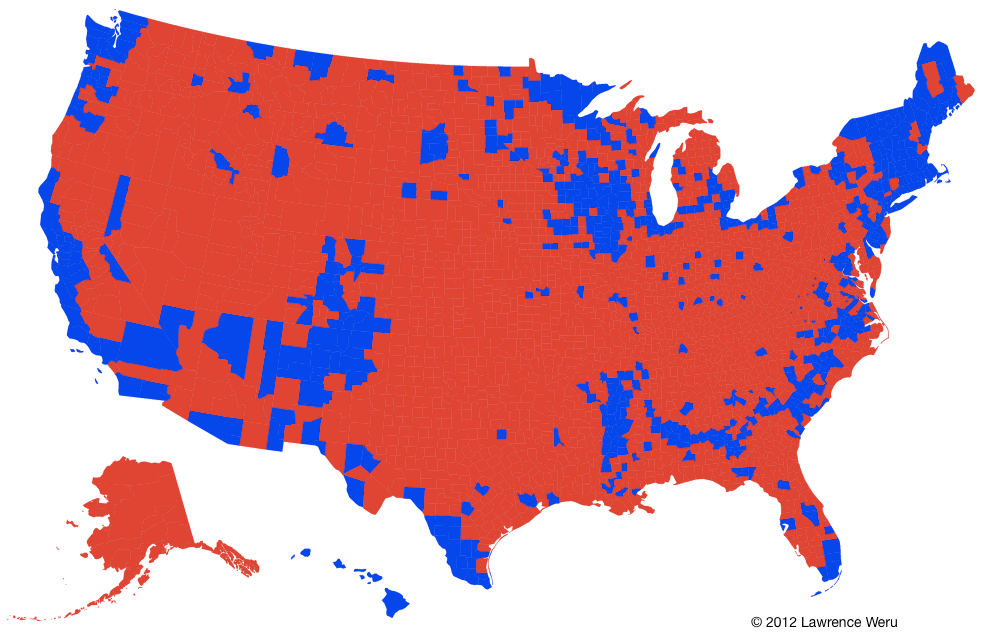
With this graph, the analyst can see that the states are a patchwork of red and blue counties. But there’s an unanswered question. Did every single person inside a given county cast the same vote? Or, were the voters within the counties divided? This graph doesn’t show this information. It just shows which choice won, even if it was by one vote. So we decide to blend each county’s red and blue vote ratios together, instead of letting the winner take all. This way if we get a pure red or pure blue county, then we know that everybody casted the same vote. And if we get a purple county, then the voters were divided. This is the result:

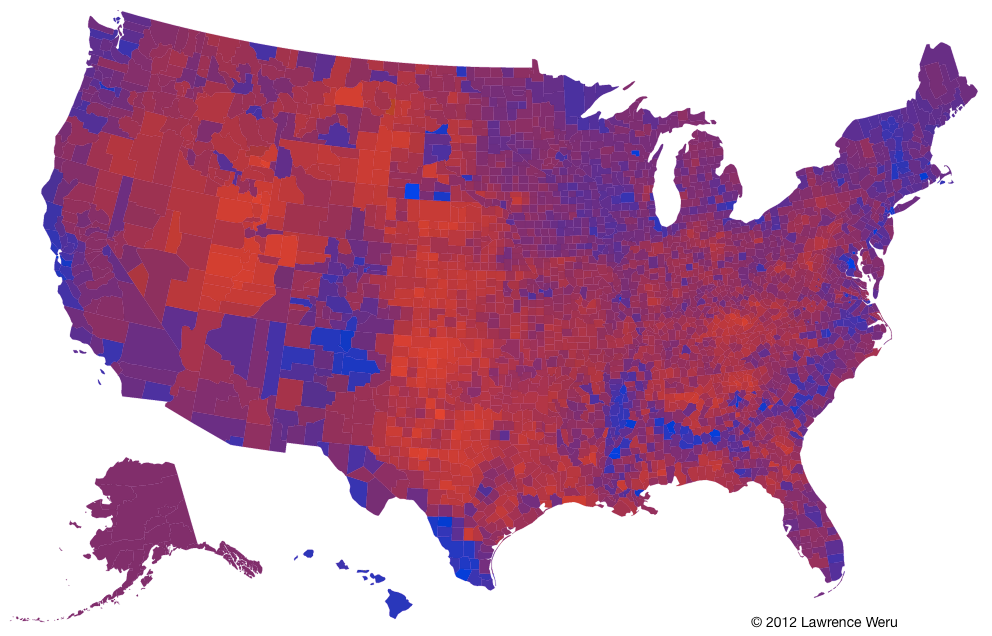
A nice blend revealing smooth purple transitions between red and blue regions. We can now see that there was hardly a landslide victory in any county. But there’s still a problem. When looking at some of the purple counties, it can be hard to decipher if the purple is leaning more towards red or blue. And it gets difficult the closer the counties get to 50/50 red/blue. In fact a R>B county can be confused as a R<B county depending on adjacent colors. In an attempt to see the margins within the counties, we end up with something that’s close, but no cigar. What’s wrong?

The problem is that in the purple map we’re no longer discerning between two distinct hues (a specific red hue and specific blue hue), but an indiscrete number of purple hues found in-between red and blue.

Magenta (I will call purple this from now on) is what our brain registers when we observe an equal mixture of red and blue light with the absence of green. We created the purple map because pure red and pure blue counties didn’t show us the vote margins. But the purple hues are nonsense. We end up looking for the quality of red-ness or blue-ness inside each purple hue to create sense. We don’t need purple at all.

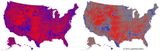
So is there a way for us to blend together red and blue hues without creating any new nonsensical hues in the process?

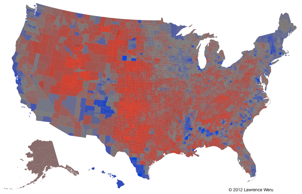
Of course! We add green, and we get a Neutralizing election map:

Interesting. How does this work? Basic color theory.

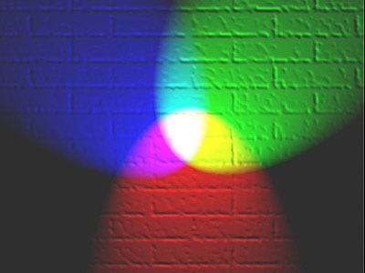
We can describe all colors as combinations of Red, Green, and Blue light. Earlier, we established that Magenta is the mixture of Red and Blue light, with the key absence of Green. But we don’t have any reservations about the absence of green for our purposes. We just want to create a gradient between red and blue. So instead of falling victim to Magenta, we can use Green to neutralize the purple-ranged colors.

For a given purple-ranged hue, if we take the weaker intensity value of that purple’s Red and Blue components — let’s call that value J — and then set the purple’s green component to that J value, the purple disappears. What’s left behind is either red or blue- whichever one was stronger in the original purple.

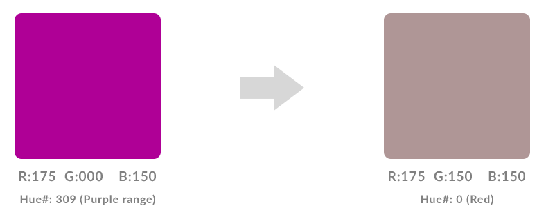
So if we take RGB[175/0/150] and Neutralize it to RGB[175/150/150], then the red hue sticks out, with some desaturation.

If we take RGB[150/0/175] and Neutralize it to RGB[150/150/175], then the blue hue sticks out, with some desaturation.

And if we Neutralize magenta, which is a 50/50 split between red and blue, the result will be a completely desaturated color since the red, green, and blue values would all be exactly the same. For example: RGB[128/0/128] Neutralizes to RGB[128/128/128].

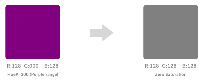
This makes sense, because when mixing together high-intensity Red, Green and Blue light, we get pure white light, which has no color saturation.

This is awesome! Thanks to this neutralizing algorithm we can pit two hues against each other and only one of the original 2 hues will be the resulting victor. No new hues! The only hues on the Neutralizing map are hue#0/hue#360 (Red) and hue#240 (Blue). So now the degree of red/blue saturation reveals the margins.

If a county even has the slightest hint of color saturation, then that color is that county’s marginal vote. There can be no dispute. This allows us to observe minute margins, such as a 49/51 red/blue split. *But there are limits to how nuanced the margins can be, since RGB’s 8-bit color-space can’t accept too many significant figures.

This Neutralizing Map can bring to our attention things we didn’t notice before — such as the blue streak in the Bible Belt isolated from the reds by a grey buffer, which doesn’t really call out to us in the Purple map.

Here’s how relative voter-turnout appears on the Neutralizing graph:

The principle behind the neutralizing map algorithm can work for all sets of colors. For example, we can neutralize a graph that has 4 fields represented by red, green, orange, and yellow. Grey would still be the intermediary between all the hues. It would just take a little extra work since we’d need to abstract away RGB.